Geometric Algebra for Geometric Deep Learning and Digital Geometry
Stéphane Breuils
Geometric Algebra
Vectors
Multivectors \( \mathbf{a},\mathbf{b} \)
Product
Geometric product
\(\mathbf{a} \mathbf{b} \)
Geometric Product
\( \mathbf{a} \mathbf{b} = \mathbf{a}\cdot \mathbf{b} + \mathbf{a} \wedge \mathbf{b} \)
\(\bullet \) invertible product and defined for vectors as:
\(\bullet \) \( \mathbf{a}\cdot \mathbf{b} \) inner product
\(\bullet \) \( \mathbf{a} \wedge \mathbf{b} \) outer product
Outer product
Briefly
- \( \mathbf{a} \wedge \mathbf{b} \)
- expresses the oriented surface spanned by \( \mathbf{a}\) et \( \mathbf{b}\)
- anticommutative
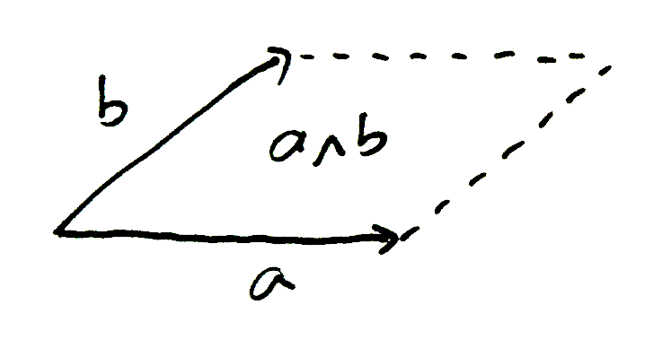
- vector \( \wedge \) vector \( = \) bivector
- expressed in the bivector subspace
Bivector
product between vectors \( \mathbb{R}^3 \)
\( \mathbf{a} = a_x \mathbf{e}_1 + a_y \mathbf{e}_2 + a_z \mathbf{e}_3 \)
\( \mathbf{b} = b_x \mathbf{e}_1 + b_y \mathbf{e}_2 + b_z \mathbf{e}_3 \)
- Defined in any dimensions
- Associative
Trivector
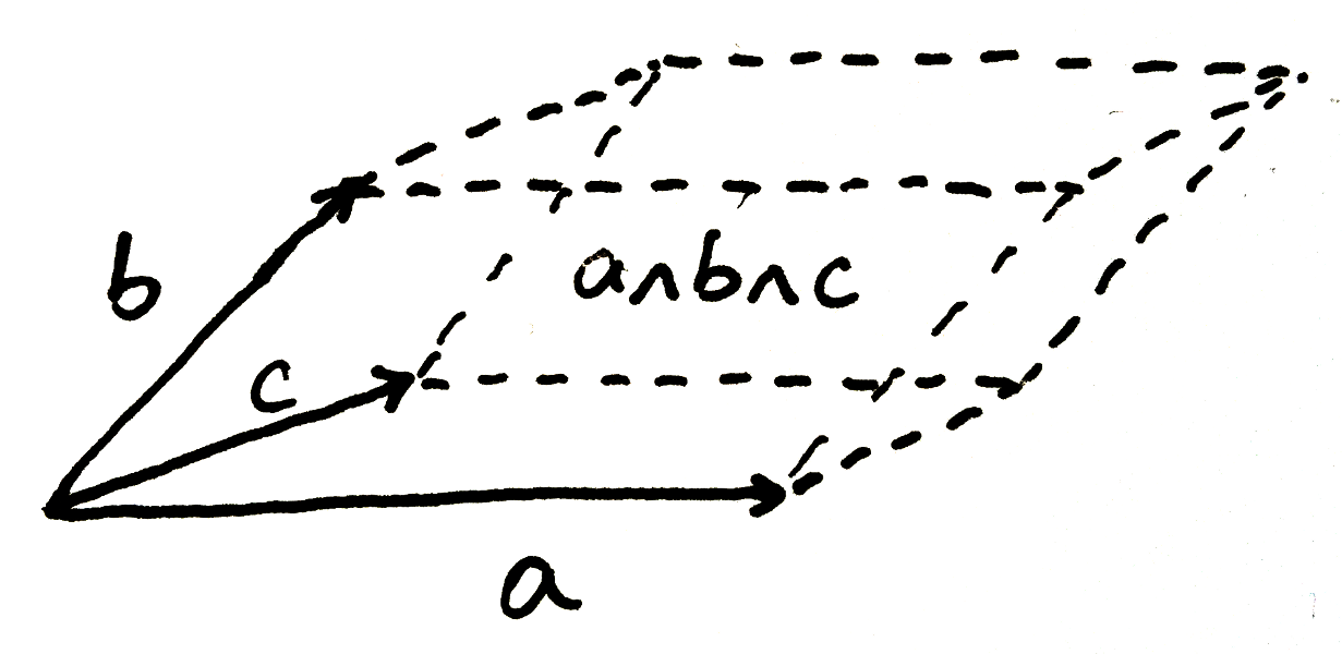
product between 3 vectors
- vector \( \wedge \) vector \( \wedge \) vector \( = \) trivector
- represents the oriented volume
- expressed in the trivector basis
k-vectors
Multivector
Grade
\( \mathbf{A}^{(2)} =a_{xy} \mathbf{e}_{12} + a_{xz} \mathbf{e}_{13} + a_{yz} \mathbf{e}_{23} \)
Inner product
Inner product
\(\bullet \) Scalar product generalisation
\(\hookrightarrow \) vector \( \cdot \) vector \(=\) scalar
\(\hookrightarrow \) \(k\)-vector \( \cdot \) \(k'\)-vector
Norm
Norm of \( \mathbf{p} \)
\( \color{gray} \left \lVert \mathbf{p} \right \rVert^2 = \mathbf{p} \cdot \mathbf{p} \)
Inverse
\(\bullet \) noted as \(\mathbf{p}^{-1}\)
Inverse of \( \mathbf{p} \)
\( \color{gray} \mathbf{p}^{-1} = \displaystyle \frac{\mathbf{p}}{\left \lVert \mathbf{p} \right \rVert^2} \)
Dual
\(\bullet \) vectors not contained in \( \mathbf{p} \)
\(\bullet \) noted \(\mathbf{p}^*\)
Dual of \( \mathbf{p} \)
\( \color{gray} \mathrm{p}^* = \mathrm{p}\mathbf{I}_n^{-1} = \displaystyle\frac{\mathrm{p}\widetilde{\mathbf{I}}_n}{\mathbf{I}_n\cdot \widetilde{\mathbf{I}}_n} = \pm\mathrm{p}\mathbf{I}_n\)
Conformal Space
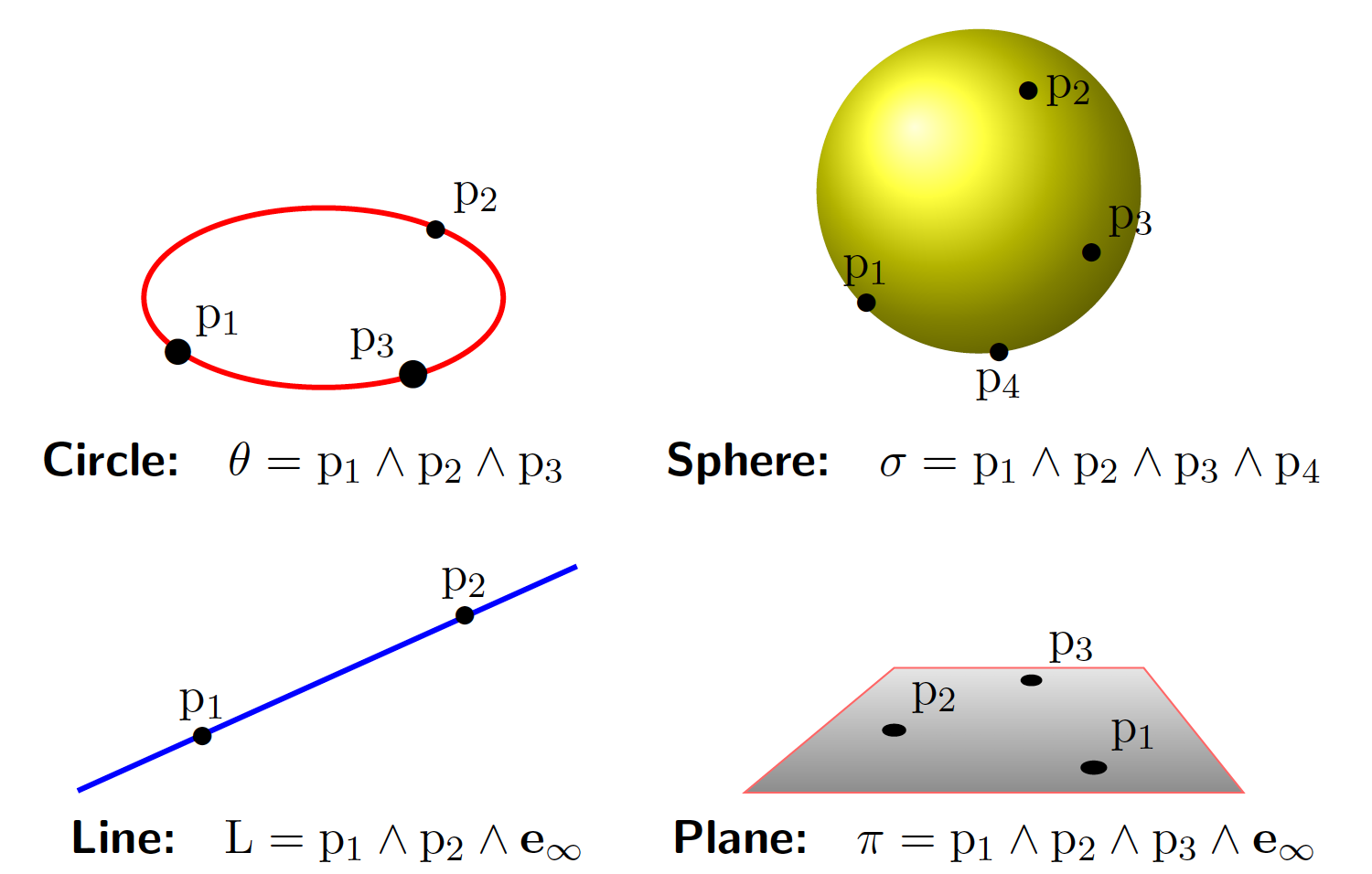
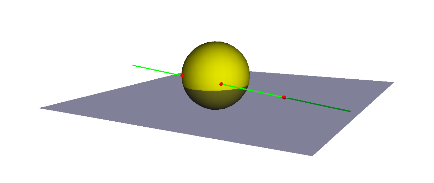
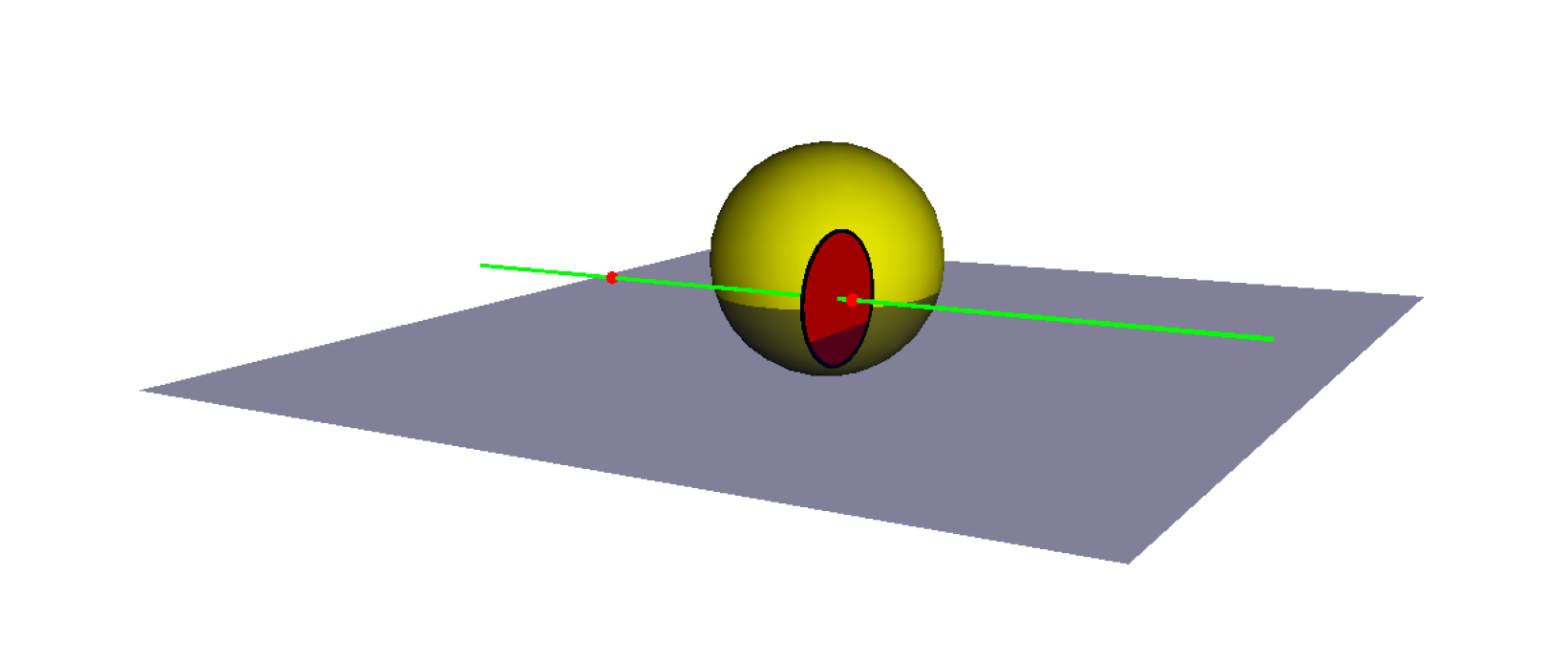
\( {\color{red}\mathbf{i}_1^{*}} = \mathbf{l}^{*} \wedge \mathbf{s}^{*} \)
\( {\color{red}\mathbf{i}_2^{*}} = \mathbf{l}^{*} \wedge \mathbf{\pi}^{*} \)
Intersections
Intersections

\( {\color{red}\mathbf{i}_1^{*}} = \mathbf{l}^{*} \wedge \mathbf{s}^{*} \)
Transformations
Reflections
\( \mathbf{y} = -\mathbf{m} \mathbf{x} \mathbf{m}^{-1} \)
- \(\mathbf{m} \) : normal vector
- \(\mathbf{x} \) : \(k-\)vector
- \(\mathbf{y} \) : result is also a \( k-\)vector
Transformations
Reflections
\( {\color{green}\mathbf{y}} = -{\color{blue}\mathbf{m}} {\color{red}\mathbf{x}} {\color{blue}\mathbf{m}^{-1}} \)
Transformations
Reflections, rotations (and translations)
\( \mathbf{Q} = \color{blue}\mathbf{m}\mathbf{n} = \cos{\frac{\theta}{2}} + \sin{\frac{\theta}{2}} \mathbf{e}_{12} \) \( (2D)\)
\( \bullet \) holds for any dimension
Reflection of \( \mathbf{x} \) with respect to the hyperplane with normal vector \(\mathbf{m} \) :
\( \mathbf{y} = -\mathbf{m} \mathbf{x} \mathbf{m}^{-1} \)
Product of \(\mathbf{m} \mathbf{n} \) is a rotation of \( \mathbf{x} \) :
Hyperbolic rotations
Inner product
\( \mathbf{Q} = \color{blue}\mathbf{m}\mathbf{n} = \cosh{\frac{\theta}{2}} + \sinh{\frac{\theta}{2}} \mathbf{e}_{12} \) \( \)
Signature of the bilinear form (1,3)
\( \mathbf{y} = -\mathbf{m} \mathbf{x} \mathbf{m}^{-1} \)
Product of \(\mathbf{m} \mathbf{n} \) is a hyperbolic rotation of \( \mathbf{x} \) :
Dual Quaternions Linear Blending for the animation of a body
Dual quaternion and 3D rigid transformation
- \( \mathbf{\tilde{q}} = \mathbf{q}_{r} + \epsilon \mathbf{q}_{d} \)
- \( \mathbf{q}_{r},\mathbf{q}_{t}\) are quaternions
- \( \epsilon \): dual number, \( \epsilon^2 =0 \)
Rotation
\( \mathbf{\widetilde{q}} = \mathbf{r} + \frac{\epsilon}{2}\mathbf{t}\mathbf{r}\)
Translation
\( \mathbf{r} = \cos(\frac{\theta}{2}) + \mathbf{u} \sin(\frac{\theta}{2}) \)
Rotation and translation
\( \mathbf{\widetilde{t}} = 1 + \frac{\epsilon}{2}\mathbf{t}\)
Dual quaternion for screw motion
- \( \mathbf{\tilde{q}} = \mathbf{q}_{r} + \epsilon \mathbf{q}_{d} \)
- \( \mathbf{q}_{r},\mathbf{q}_{t}\) are quaternions
- \( \epsilon \): dual number, \( \epsilon^2 =0 \)
Transformation of points \( 1+ \epsilon \mathbf{p} \)
\( \mathbf{\widetilde{l}'} = \mathbf{\widetilde{q}} (\mathbf{\widetilde{l}}) \mathbf{\widetilde{q}}^* \)
Transformation of line : \( \mathbf{\widetilde{l}} = \mathbf{l} + \epsilon \mathbf{m} \) ( \( \mathbf{m} \) moment of the line )
\( \mathbf{\widetilde{p}}'= \mathbf{\widetilde{q}} (1+ \epsilon \mathbf{p} ) \mathbf{\widetilde{q}}^* \)
Dual quaternion Blending (Kavan, Leclerc)
- \( \mathbf{\tilde{q}} = \mathbf{q}_{r} + \epsilon \mathbf{q}_{d} \)
- \( \mathbf{q}_{r},\mathbf{q}_{t}\) are quaternions
- \( \epsilon \): dual number, \( \epsilon^2 =0 \)
Interpolation (blending) of \( n \) nodes (5 in the implementation )
\( \mathbf{w}(v, n) \in \mathbb{R} \)
Dual quaternion Neural Network
Activation, Pooling
\( x ^{(l+1)} = ψ(z^{(l+1)}) = ψ(W^{(l)}x^{(l)} + b^{(l)} ) \)
\( \bullet W^{(l)}\) Unit dual quaternion weights
\( \bullet x^{(l)},b^{(l)}\) Dual quaternions
\( \bullet \psi \) Dual quaternion function or split activation function
Dual quaternion and pytorch implementation
https://github.com/sbreuils/ga-dq-pytorch.git
Dual Quaternion Neural Network
Attention mechanism (Pöllenbaum,Schwung 2022)
Queries : Dual quaternion nodes
Keys : Reference dual quaternions
In Vector Valued Neural network, attention score is computed as the softmax of the dot product between keys and the query
\( \hookrightarrow \) Key idea : relative error between dual quaternions \(\mathbf{\tilde{q}_1},\mathbf{\tilde{q}_2} : \)
Quaternion Convolution Network
QCNN
Quaternion Convolutional Neural Network (QCNN)
Quaternion Kernel : \( \mathbf{w} (L \times L)\)
Input quaternion : \( \mathbf{x} (N \times N)\)
Quaternion convolution
\( \mathbf{x}'_{kk'} = \sum_{l=1}^L \sum_{l'=1}^L w_{l,l'} (x_{k+l,k'+l'})w_{l,l'}^* \)
Dual Quaternion network
SE(3) equivariant Neural network
DQNN
\( \mathbf{\widetilde{q}} \mathbf{\widetilde{x}}\mathbf{\widetilde{q}}^* \)
DQNN
\( \mathbf{\widetilde{x}} \)
\( \mathbf{\widetilde{f}}(\mathbf{\widetilde{x}}) \)
\( \mathbf{\widetilde{q}}\mathbf{\widetilde{f}}(\mathbf{\widetilde{x}})\mathbf{\widetilde{q}}^* \)
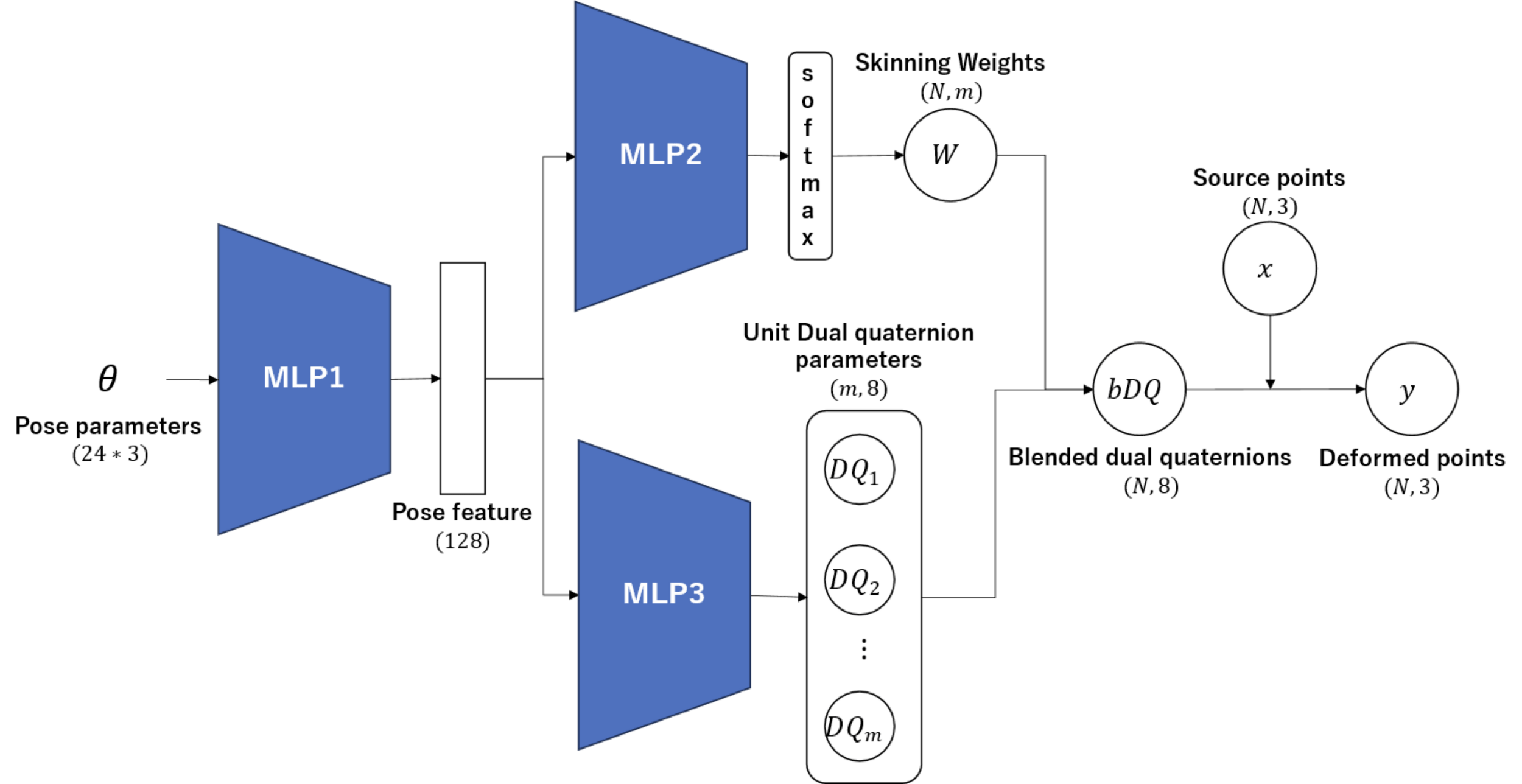
Dual Quaternion Blending Neural network

Network for the moment
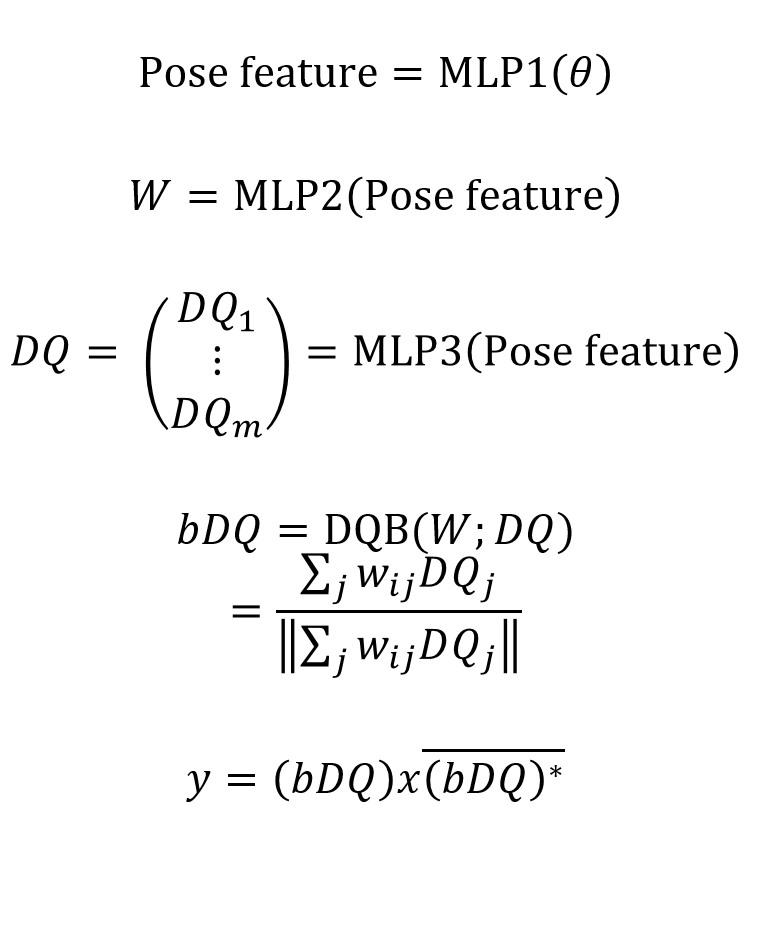

Network for the moment


\( J(x,y,bDQ) = \sum_i |SDF(y_i)| + \lambda \sum_j ||bDq_j || \)
Some results
Ours
Ground truth
Kitamura et al.
Dual Quaternion Network : Symmetry equivariant ?
Dual quaternion does not represent composition of reflections with respect to planes
Get symmetry equivariant NN
with geometric algebra
Equivariance to both grade projection \( (\_ )^{(m)}\) and polynomials \( F \)

Geometric Algebra and bijective digitized transformations
Bijective digitized transformations
Operators
Reflections to rotations and translations
\( \bullet \) Reflections \( \mathcal{U}^{m} \)
\( \bullet \) Digitized operator \( \mathcal{D} \)
\( \bullet \) Digitized Reflections \( \mathcal{R}^{\mathbf{m}}\)
Digitized cell
Voronoi cell equivalent definition
\( \mathcal{C}_{1}(\mathbf{0})\)
\( \mathcal{C}_{1}(\mathbf{t})\)
\( \mathbf{t} = 3 \mathbf{e}_1 + 2 \mathbf{e}_2\)
Digitized cell
\( \bullet \) Reflection
\(\mathcal{C}_{\frac{\mathbf{m}}{||\mathbf{m} || }} (\mathbf{0}) \)
Voronoi cell equivalent definition
Bijective digitized reflections in 2D
\( \bullet \) Idea: use bijectivity condition of digitized rotations
(Jacob, Andres, Nouvel, Roussillon, Coeurjolly)
\( \bullet \) Geometric algebra, rotation of angle \(\theta\) of an object \(\mathbf{x}\):
Bijective transformations from composition of bijective reflections
Motivation : Sparse angular distribution of bijective digitized reflection and rotations
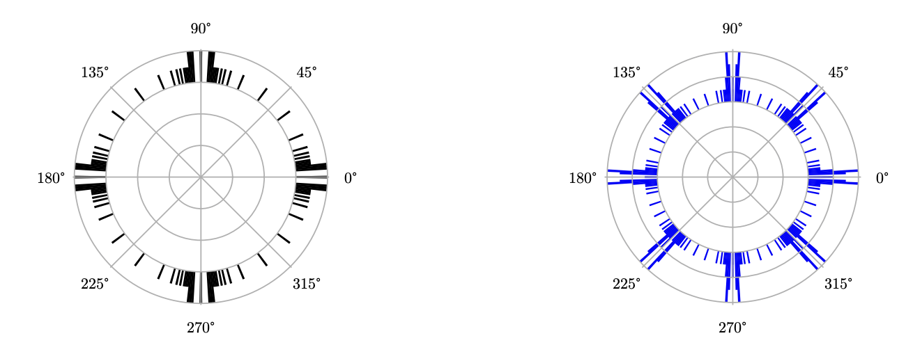
Get more bijective transformations
Angular distribution of the composition of bijective digitized reflections
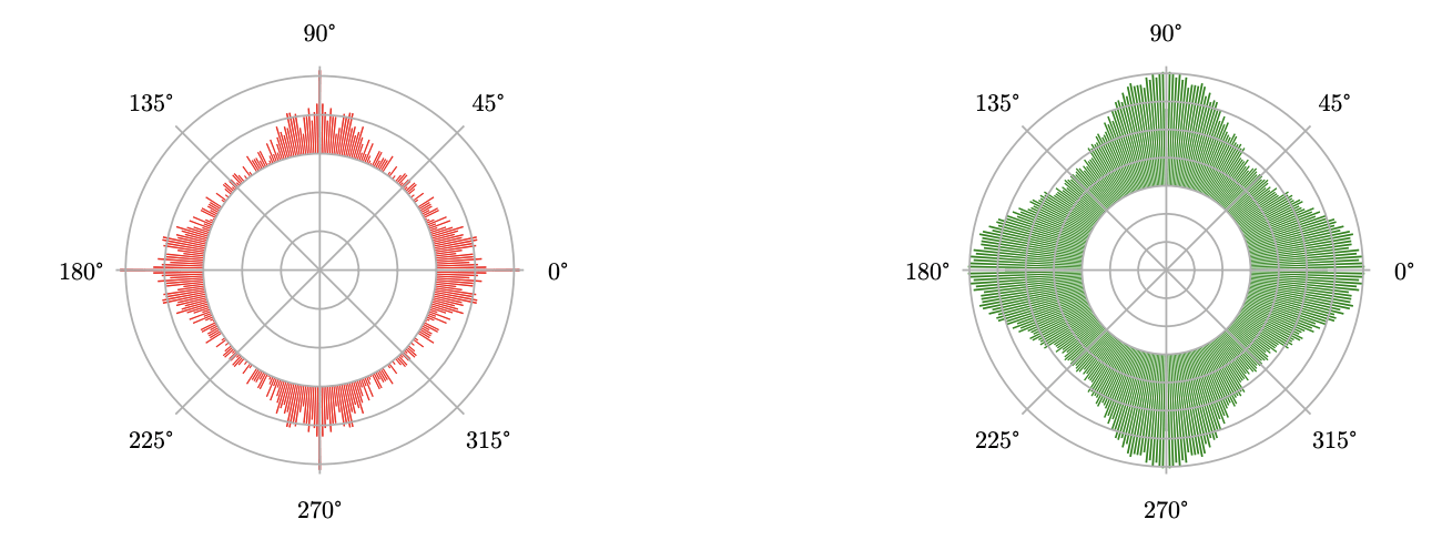
2 bijective digitized reflections
4 bijective digitized reflections
How to Choose the bijective composition ?
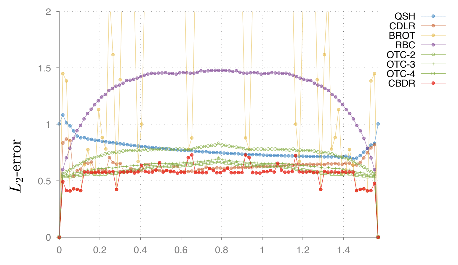
For each rotation angle \(\theta\), we thus compute the composition that minimizes the Linf error with respect to the real rotation
Several composition leads the same resulting rotation angle but can induce
different L2 and Linf errors
Composition of Bijective Digitized reflections
In 3D
\( \bullet \) Pluta, Romon et al proposed an algorithm to certify bijective rotations with Lipschitz quaternions
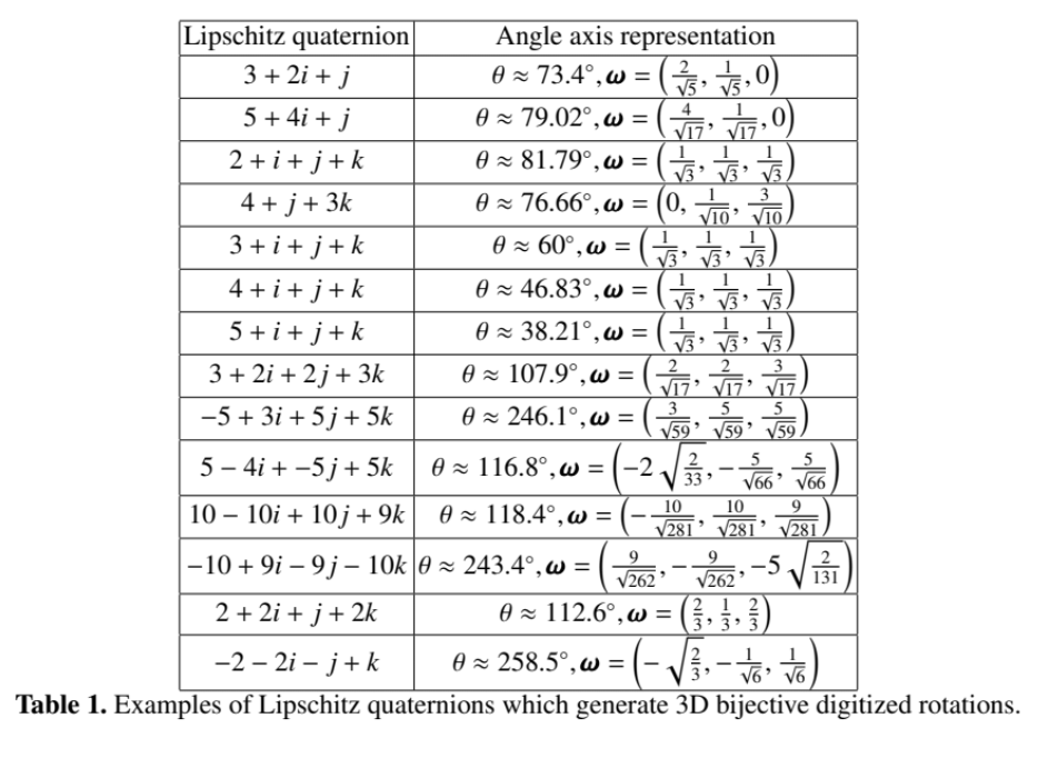
Lipschitz quaternion and conjecture of 3D bijective digitized reflections
\( \bullet \)Given a normal vector \( \mathbf{m} \), compute the geometric algebra rotation \( R = \mathbf{e}_1 \mathbf{m} \)
\( \bullet \)Since scalar and bivectors \(\mathbb{R} \oplus \bigwedge^2 \mathbb{R}^3 \cong \) division ring of quaternions
\( \rightarrow \)Certification of \( R \) using Pluta, Romon and Kenmochi algorithm
Conjecture 2
\( \bullet \) characterisation of 3D bijective digitized reflections is the extension of 2D bijective digitized reflections
Conjecture 3
\( \bullet \) Any bijective digitized rotation in 3D can be defined as the composition of one bijective digitized reflections and one reflection with respect to